Neural Networks Through Magnifying Glass

Last week in our ML series, we introduced the process of training artificial neural networks—its phases, data splitting, and the importance of monitoring the training process. Today, we want to delve deeper and analyse what happens inside a neural network during a single training epoch. Let’s get started!

One Step Forward, One Step Back

First and foremost, it’s essential to note that while the general concept of training neural networks is relatively consistent, there are many variations. Today, we will discuss one of the simplest methods—adjusting the model’s weights and biases after each individual sample from the training dataset is presented (in the literature, this approach is known as stochastic gradient descent – SGD).

With that said, let’s explore what happens inside a neural network during a single training epoch:

1. A specific sample (a vector of numbers) from the training dataset is loaded into the model’s input layer.
2. The input data passes through each layer of the network, undergoing various operations, alternating between linear and non-linear transformations.
3. The output layer produces probabilities of the input sample belonging to each of the considered classes (each neuron in the output layer represents one class).
4. The loss function evaluates how much the model “misclassified” the input sample based on the known label (the actual correct class).
5. Subsequently, the gradient is calculated, which is the derivative of the loss function with respect to all network parameters (weights and biases). In a simplified sense, this multi-dimensional derivative allows us to determine how much a particular parameter influenced the value of the loss function (i.e., the error made by the model in its current state) and how it should be corrected.
6. The network parameters are adjusted based on the calculated gradient.

Steps 1-4 are often referred to as the forward pass, and steps 5-6 are known as the backward pass.

Neural Networks Layers – How to Construct Them?

It’s essential to pay attention to one more aspect of neural network architecture. While hidden layers can contain any (within reason) number of neurons, it is common to choose powers of 2 for their size. However, when it comes to input and output layers, there are some specific rules to follow:

• The input layer must have as many neurons as the input vector’s elements. Remarkably, the input layer is the only exception where none of the operations described in the previous article takes place. This is because each neuron in this layer only receives one value, corresponding to the n-th element of the input vector.

• The output layer must contain as many neurons as there are classes in the task. Each neuron in the output layer represents one of these classes, and, in essence, it estimates the probability of the input sample belonging to that specific class (usually as a probability in range (0, 1).

Let’s take a jump back to the figure from one of our previous articles of this series:

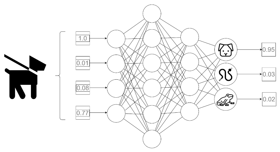
Fig. 1: A simplified example of a forward pass

Now, let’s take a closer look at what happens during the forward pass through the hidden layers of the network:

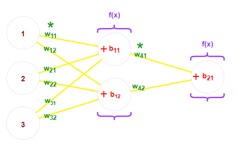
Fig. 2: A close-up look on neural networks parameters: weights are green, biases are red (roses are too), activation functions are purple.

• The values returned by neurons in the input layer “travel” through connections to each neuron in the next layer. Each connection has a weight, W, through which the input value is multiplied.
• At the input of the next-layer neuron, all incoming values multiplied by their respective weights are summed. This sum is also added to the bias value, B, specific to that neuron.
• The resulting sum is passed through an activation function, denoted as A. The purpose of such a function is to break the linearity of the operations conducted. What does this mean?

Notice that the operations conducted so far (multiplication and addition) linearly modify the input values. If we continued to treat data this way, each subsequent layer would be a linear transformation of the previous layer’s output. This output is, in fact, a result of linear operations. Mathematics leaves no doubt in this regard—composing linear functions, regardless of their number, is still just a linear function! It means that without introducing activation functions that break the linearity of our structure, the entire complex neural network could ultimately be replaced by… a single function of the form f(x) = ax + b. While linear functions are surprisingly powerful statistical tools, constructing them through elaborate, artificial neural networks might sound a tiny bit like an overkill.

Neural Networks – How About This Activation?

Now, let’s talk about activation functions:

• Activation functions in hidden layers: 
  • the most commonly used activation function in hidden layers is ReLU (Rectified Linear Unit): 

f(x) = max(0, x). 

This function maintains linear dependence for values greater than or equal to zero, while rounding off all negative values to zero.

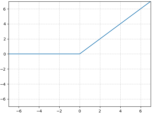
Fig. 3: Plotted ReLU

• Activation function of the output layer: 
  • the choice of the activation function in the output layer depends on the task. For binary classification, the sigmoid function is commonly used. It returns values in the range (0, 1), and values below 0.5 are usually interpreted as belonging to one class, while values above 0.5 are associated with the other.

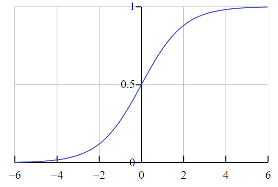
Fig. 4: Plotted sigmoid (src: Wikipedia.org)

• Regarding multi-class problems, on the other hand, the softmax function is often employed. It transforms the values of neurons in the output layer to ensure they sum up to 1. This function is unique because it operates on all neurons in the output layer simultaneously, rather than a single neuron.

Confronting the Truth – Loss Function and Backpropagation

We’ve achieved results; now it’s time to check how far they are from the truth. The loss function helps us determine how much error our network has made by comparing the obtained results with the ground truth. Commonly used loss functions include cross-entropy and categorical cross-entropy, but delving into the mathematical details is beyond the scope of this article.

The final step in the parameter adjustment phase of an epoch is backpropagation. It involves calculating the derivative of the loss function for each parameter in the network. This derivative tells us in which direction and to what extent each weight or bias should be adjusted to bring the result closer to the truth. After computing this multi-dimensional derivative (the gradient) for all trainable network parameters, their values are updated (how drastically depends on the chosen learning rate).

That’s all for today! See you next week when we’ll take a closer look at how the training could be improved and how do neural networks look from a cybersecurity perspective. Take care until then!